How to Build a Simplified MICE Imputation Workflow in R
Why rebuild MICE by hand?
Multiple imputation by chained equations (MICE) is a familiar tool for handling missing data, but its inner workings can feel opaque. The author set out to recreate a simplified version in R, learning through mistakes and help from others. The result came close to the mice package—though the author is careful to say that could be luck. This is a useful exercise in understanding the machinery, but it isn’t a claim to have recreated the package itself.
The appeal of MICE is easy to see. Replacing each missing value with a single estimate, such as a mean, hides the uncertainty in that estimate and can make standard errors too small. MICE instead creates several completed datasets, drawing plausible values for the gaps. You analyse each dataset, then combine the results using Rubin’s rules.
“Chained equations” describes the iterative process: a model predicts each incomplete variable from the others, then the updated values feed into the next model. The sequence cycles through the variables repeatedly. That sounds almost magical when you first use it; writing a small version yourself is a good way to see where the magic comes from.

A small experiment, with clear limits
The walkthrough starts by simulating 1,000 observations in R. It creates three continuous predictors, two binary predictors, and a binary outcome. Missingness is then introduced under three mechanisms: p1 and p3 use MCAR; p2 and p4 use MAR, with missingness depending on p1 and, for p4, p2; p5 uses MNAR, with missingness depending on its own value. The outcome remains observed.
That setup gives the author a known data generating process to work from, then a deliberately damaged dataset to impute. It’s a practical teaching choice: the reader can follow the code from complete data through missingness and reconstruction. But the example is explicitly a simplified implementation, and its close resemblance to the package is not evidence that every detail matches.
What the implementation does
The R code records the row and column of every missing entry, along with each variable’s data type. It seeds those gaps with random starting values, then cycles through the incomplete columns. For each column, it bootstraps rows where the value is observed and fits a regression using the other variables—including the outcome—as predictors. Continuous variables use linear regression; binary variables use logistic regression. Predictions receive random variation: residual noise for continuous values, and probability-based 0/1 draws for binary ones.
The script runs ten iterations per chain and keeps the last set of imputations. It repeats that process for ten chains, producing ten completed datasets. A logistic regression of the binary outcome on p1 through p5 is fitted to each dataset, and the results are intended to be pooled. The author’s outline says to average coefficients and use Rubin’s rules for standard errors.
Here’s the thing: the value of this exercise is less the claim that MICE is now “understood” than the concrete view it gives of the steps—initial fills, repeated conditional models, multiple completed datasets, and pooled analysis. The author also flags that the code is messy and may contain redundancies, and notes that the underlying OLS and maximum-likelihood routines are not being rebuilt from scratch. The first fitted model is presented as looking reasonable, but this opening section doesn’t yet establish how well the imputations recover the known data.
The article proceeds through five topics: what MICE is, simulating the data, the imputation procedure and pooling, opportunities for improvement, and lessons learned. It also points readers to a separate explanation of missing data mechanisms.
Pooling the imputations
The key distinction is that multiple imputation pools model results, not the imputed datasets themselves. For each of the six coefficients, the code below averages estimates across 10 fitted models, then combines within-model variance with between-model variance. It uses Barnard–Rubin degrees of freedom to set the 95% confidence interval’s t value.# assess the point estimate of coefficient
coef <- 1:6
fit_list <- 1:10
temp_coef <- c()
# temp_coef_var <- c()
model_coef <- c()
model_coef_var <- c()
for (i in coef) {
for (j in fit_list) {
temp_coef[j] <- fits[[j]]$coefficients[[i]]
}
model_coef[i] <- mean(temp_coef)
model_coef_var[i] <- var(temp_coef)
}
# assess the pooled SE to construct 95% CI of the coefficients
se <- do.call(rbind, map(.x = fits, ~ tidy(.x) |> pull(std.error))) |> as_tibble()
within_var <- colMeans(se^2)
between_var <- model_coef_var
total_var <- within_var + between_var + between_var / length(fit_list)
final_se <- sqrt(total_var)
# degrees of freedom (Barnard–Rubin)
lambda <- (1 + 1/length(fit_list)) * between_var / total_var
df_com <- 1000 - 6
df_old <- (length(fit_list) - 1) / lambda^2
df_obs <- (df_com + 1) / (df_com + 3) * df_com * (1 - lambda)
degfree <- df_old * df_obs / (df_old + df_obs)
tval <- qt(0.975, degfree)
mice_coef <- tibble(term = fits[[1]] |> tidy() |> pull(term), estimate = model_coef, std.error = final_se, tval = tval,
conf.low = estimate - tval * std.error, conf.high = estimate + tval * std.error) |>
select(-tval) |>
mutate(method = "our_mice")
To check the hand-built pooling against the established implementation, the article fits the same logistic regression with R’s `mice` package and pools its results:
library(mice)
imp <- mice(df_miss, m = 10, maxit = 10, seed = 1, printFlag = FALSE)
fit <- with(imp, glm(outcome ~ p1 + p2 + p3 + p4 + p5, family = binomial))
actual_mice_coef <- tidy(pool(fit), conf.int = TRUE) |>
select(term, estimate, std.error, conf.low, conf.high) |>
mutate(method = "actual_mice")
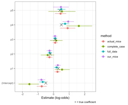
The comparison also includes a fit on the full data and one using complete cases. The plotted reference values are the data-generating coefficients: an intercept of −0.5, then 0.3, −0.2, 0.1, 0.5, and 0.4 for p1 through p5.
## function to grab stats
grab_stats <- function(df, method) {
model <- glm(outcome ~ p1 + p2 + p3 + p4 + p5, df, family = "binomial")
coef <- model |> tidy(conf.int = T) |> select(-statistic, -p.value) |> mutate(method = method)
return(coef)
}
## full data
full_data_coef <- grab_stats(df, "full_data")
## complete case
cco_coef <- grab_stats(df_miss, "complete_case")
## complete case analysis
all_coef <- rbind(mice_coef, full_data_coef, cco_coef, actual_mice_coef)
## truth
truth <- tibble(term = c("(Intercept)", "p1", "p2", "p3", "p4", "p5"),
truth = c(-0.5, 0.3, -0.2, 0.1, 0.5, 0.4))
## visualize all
all_coef |>
ggplot(aes(x = estimate, y = term, color = method)) +
geom_vline(xintercept = 0, linetype = "dotted", colour = "grey60") +
geom_pointrange(aes(xmin = conf.low, xmax = conf.high),
position = position_dodge(width = 0.6)) +
geom_point(data = truth, aes(x = truth, y = term),
inherit.aes = FALSE, shape = 4, size = 4) +
labs(x = "Estimate (log-odds)", y = NULL,
caption = "× = true coefficient") +
theme_bw()

What still needs work
A close match with `mice` is a useful validation, but it doesn’t settle every modeling choice. The next steps are to learn posterior sampling, try predictive mean matching—the `mice` default, which draws from observed values to keep imputations in realistic ranges—speed up and tidy the code, and run sensitivity analyses. The suggested code improvements are to vectorize `missing_fill()`, keep state in lists instead of global variables, and pass the random generator explicitly.What the exercise taught
The author describes a bumpy process that began on 10/9/26: an initial attempt incorrectly averaged the imputed datasets, followed by a correction to pool model estimates properly. The work led to a practical understanding of `mice`, `map2_dfc`, Rubin’s pooling rules, the total-variance formula, and Barnard–Rubin degrees of freedom. The author credits repeated conversations with an LLM as a tutor in reaching the correct technique. If you’d like to comment or read more, visit the author’s blog. You can also follow them on BlueSky, Twitter, GitHub, or Mastodon, or get in touch about collaboration.
To leave a comment for the author, visit r on Everyday Is A School Day.
R-bloggers.com offers daily email updates about R news, tutorials about learning R, and other topics. Visit R-users.com to post or find an R or data science job. To share your own content on R-bloggers, submit your blog or, if you don’t have one, use r-posts.com.
Continue reading:My Messy Notes of Learning MICE From Scratch