Simpson’s Paradox in Python: Why Exam Difficulty Reverses Pass Rate Comparisons
Why the pooled result tells a different story
Program B leads the simulated data by more than 30 percentage points when all students are counted together. Yet within both easy and hard exams, Program A has the higher pass rate. That reversal is the central lesson of Simpson’s paradox: a pooled comparison can point in the opposite direction from every comparison made within relevant subgroups.
Here, the shift comes from exam difficulty and the way students are distributed across programs. Program A sends most of its students to hard exams, where passing is less likely. Program B sends most of its students to easy exams. The resulting aggregate rates reflect both students’ pass rates within each difficulty group and the different weights those groups receive.
The example is simulated in Python, with NumPy generating outcomes, pandas summarizing them, statsmodels fitting logistic regressions, and plotnine producing a figure. The code runs inside an R Markdown document through reticulate. For analysts, the useful point is not simply that an aggregate can mislead. It’s that a regression coefficient and a raw rate answer different questions when group composition varies.
The design builds the reversal in
The simulation assigns 20,000 students to programs A and B and to easy or hard exams. Program A has 1,000 students taking easy exams and 9,000 taking hard exams. Program B has the inverse distribution: 9,000 take easy exams and 1,000 take hard exams.
| Program | Exam difficulty | Students | Pass probability |
|---|---|---|---|
| A | Easy | 1,000 | 90% |
| A | Hard | 9,000 | 40% |
| B | Easy | 9,000 | 80% |
| B | Hard | 1,000 | 30% |
Within either exam category, A has a 10-point advantage in the specified pass probabilities. But the overall groups have very different mixes of exam difficulty. A’s cohort is 90% hard exams; B’s is 90% easy exams. Since easy exams have higher pass probabilities for both programs, that difference in mix is large enough to overturn the within-group comparison.
Each student’s outcome is generated independently as pass or fail using the probability assigned to that student’s program and exam difficulty. The random seed is fixed at 2026, making the simulation reproducible. The group sizes are set in advance, while the observed numbers of passes vary due to random sampling.
What the simulated rates show
In the generated sample, Program A’s easy-exam pass rate is 88.60%, compared with 79.66% for B. Among hard-exam takers, A reaches 39.29%, while B records 31.00%. A leads in both comparisons.
Pooling the groups flips the ranking. A’s 10,000 students pass at a rate of 44.22%; B’s 10,000 students pass at 74.79%. That headline comparison describes the cohorts as they were assembled, including their unequal exposure to exam difficulty. It doesn’t describe a like-for-like comparison at a fixed difficulty level.
A plot makes the split visible: two panels compare pass rates within easy and hard exams, while a third shows the combined rates. The source figure is retained here.
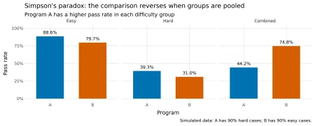
Figure 1: Pass rates within difficulty groups and after pooling students.
The weights explain the reversal
An aggregate pass rate is a weighted average of subgroup rates. The weight for each exam category is its share of students in that program. Because A and B have sharply different exam mixes, their subgroup rates contribute in different proportions.
For A, easy exams account for one tenth of students and hard exams for nine tenths. Using the observed counts, the calculation is: (1,000 / 10,000) × (886 / 1,000) + (9,000 / 10,000) × (3,536 / 9,000) = 0.4422, or 44.22%.
For B, the weights are reversed: nine tenths easy and one tenth hard. Its observed aggregate is (9,000 / 10,000) × (7,169 / 9,000) + (1,000 / 10,000) × (310 / 1,000) = 0.7479, or 74.79%.
The reversal isn’t an accident introduced by the random draw. It’s already present in the probabilities used to generate the data. A’s expected rate is 0.10 × 0.90 + 0.90 × 0.40 = 0.45. B’s is 0.90 × 0.80 + 0.10 × 0.30 = 0.75. Sampling produces the observed rates around those expectations; the uneven weights create the direction of the result.
Regression changes the question
A logistic regression with program as its only predictor estimates a positive coefficient for B relative to A: 1.3197 on the log-odds scale. That aligns with the pooled rates. The reported p-value is below 0.001, so the model finds a statistically clear association in this simulated sample. But statistical precision doesn’t change what the model compares: students in the two programs as they appear in the data, with their different exam mixes.
Adding exam difficulty changes the program coefficient to -0.4760. The model now compares programs while holding difficulty constant, and the estimated direction agrees with the within-category rates. Difficulty also has a large negative coefficient, -2.2809 for hard exams relative to easy exams. These adjusted estimates make the composition effect easier to see, though the coefficient remains a model-based comparison on the log-odds scale, not a pass-rate difference in percentage points.
Difficulty functions as a confounder in this constructed example because it is associated with program membership and affects the chance of passing. Leaving it out blends differences in exam difficulty with the program comparison. Including it provides a conditional comparison among students taking exams of the same difficulty.
Interpretation depends on the data-generating process
Simpson’s paradox is a warning to inspect group sizes alongside group rates. An aggregate is not simply a neutral summary of subgroup performance: its weighting reflects who appears in each group. When the mix differs, the pooled number can answer a practical question about the actual cohorts while obscuring the comparison someone may intend to make.
That doesn’t mean analysts should automatically divide data into every available subgroup or adjust for every measured variable. A reversal by itself doesn’t establish causation, and adjustment choices depend on how variables relate. Conditioning on a collider, for example, can introduce bias. The relevant structure needs to be considered before choosing a model.
For this simulation, the concrete takeaway is straightforward: report the composition, inspect rates within meaningful categories, and be explicit about whether a result is pooled or adjusted. The next question is not just which program has the higher pass rate, but which comparison fits the decision being made.