How to Choose Causal Machine Learning Methods for Intervention Analysis
Start with the data, not the algorithm
The main lesson from these simulations is less about which model wins than about when the data can support a causal claim at all. A flexible algorithm can handle complex patterns; it can’t repair a missing confounder or tell you which variables belong in the analysis. Across nine simulated settings, each repeated 40 times with a known true effect, the design and the question mattered as much as the choice of method. For data scientists deciding whether an intervention—a call, discount, or campaign—works, the results point to five practical lessons: 1. **Get the causal setup right first.** If an important influence is missing, or a variable is incorrectly included, every method can be wrong. Domain knowledge matters; in some cases, an instrument can help (Cases 4 and 5). 2. **For an average effect, causal ML has a clear advantage when confounders act nonlinearly.** In that setting, a linear model is biased while Double ML comes close to the true effect. The gain comes from its two-stage design—adjust first, then estimate—not from any one machine-learning algorithm (Case 3). 3. **Risk isn’t treatment effect.** Targeting customers most likely to cancel can perform worse than random selection: those customers may already be difficult to retain. In Case 7, the top-30% uplift was 0.037, below chance. 4. **Finding the right people is easier than estimating the effect’s size.** A GLM can rank units correctly while substantially misjudging how large the effect is (Case 9). 5. **Causal forests earn their keep when effects vary and their pattern is unknown.** They perform well when the goal is to estimate an effect for each unit. In simpler settings, a correctly specified GLM does better (Cases 6, 8 and 9).How to use the guide
The guide that follows starts with the decision you need to make, checks whether the data can support a causal estimate, and only then recommends a method. That order is deliberate: no estimator can rescue a comparison that lacks a credible basis. The next section offers decision trees and a recommendation table. The methodology section defines the terms, sets out the methods and their tradeoffs, and discusses how to assess results when the true effect is unknown. The simulation section presents all nine cases, with data, results, and a lesson from each. Numbers in square brackets refer to the references at the end.Choose a method by asking the right question
The guide’s examples use a fictional online fitness subscription service, but “unit” can mean a customer, person, contract, or branch—whatever receives the intervention. Start by distinguishing among three goals: estimating an average effect (ATE), ranking units by their likely response, or estimating the effect for each unit (CATE). Ranking can be useful even when the model gets the effect’s magnitude wrong; cost-benefit decisions for individual units usually need that magnitude too. There’s also a separate question that’s easy to confuse with treatment effect: who is likely to cancel without intervention? A GBM can estimate that risk. It doesn’t tell you whom a retention offer will help. [Image: decision guide](/articles/6336/siT5qmJa5awhdMJl9gsVQOEvuCrXZvLh.webp) Blue marks a question, green a recommendation, and red a stopping point.First establish what the data can identify
Random assignment, as in an A/B test or lottery, makes treated and untreated units comparable in expectation. If the business chose who received treatment, the groups may already differ. The analysis then depends on whether the data capture the factors that influenced both treatment and outcome. A confounder is one such shared cause: age, for example, might affect both who gets a retention call and the chance of cancellation. It belongs in the model if measured, and its form matters if its influence is nonlinear. A mediator sits downstream of treatment: a call might prompt a customer to set up a training plan, which in turn affects whether they stay. If the goal is the total effect of the call, controlling for the plan would remove part of that effect. A collider is a shared consequence of treatment and outcome; conditioning on it can create a misleading relationship between them. The practical rule is simple, though applying it takes knowledge of the process: include relevant causes that exist before treatment; don’t automatically adjust for variables that arise afterward. The data alone won’t tell you which role a variable plays. Cases 4 and 5 show why that judgment matters. [Image: causal diagram](/articles/6336/cbZPiRiN6DX6BFHSkgt254MDjtzVnV3Y.webp) [Image: causal diagram](/articles/6336/OVeFr47GavjlDYcwYaZiJspksaPqBy5K.webp) [Image: causal diagram](/articles/6336/nnE2Ohq2BfxCi1vy73pRsmG0hanTBroj.webp) If you suspect a confounder is missing, the data can’t prove its absence. A placebo test can expose some problems: an outcome the treatment cannot affect should show an estimated effect of zero. An E-value describes how strong an unmeasured confounder would need to be to explain away an estimate. DoWhy can run sensitivity checks automatically; DAGitty can help map a causal process and identify adjustment variables. The references include an overview of good and bad controls [19], guidance on E-values [20], DAGitty [26], and DoWhy [27]. An instrument—a random nudge that changes treatment but affects the outcome only through treatment—can sometimes identify an effect despite an unmeasured confounder. Two-stage least squares (2SLS) suits a constant effect; an instrumental forest can estimate varying effects. But instrument validity can’t be established from the data alone. If there’s no valid instrument, report an association rather than a causal effect. Before-and-after data or a treatment threshold may allow difference-in-differences or regression discontinuity, though those methods aren’t simulated here. Overlap is another requirement: each relevant group needs treated and untreated units. Check the propensity distribution. If propensities approach zero or one, narrow the target population to the region where both treatment states occur; otherwise, weighting methods such as AIPW can become unstable. The simulations don’t test that restriction.Match the method to the decision
Once the identification assumptions hold, the choice depends on the assignment process, the complexity of the data, and whether you need an average, a ranking, or a unit-level effect. The recommendations below are grounded in the simulations, so treat them as evidence from these cases rather than a universal leaderboard. [Image: method decision tree](/articles/6336/njA7im9YghXCMyrt4zMTSf9WGJV5t9F5.webp) For a randomized test, a mean comparison estimates the average effect; adding covariates to a linear model can help reduce variance. With only a few hundred observations, be cautious about trying to rank people: if there’s little evidence that effects vary, assigning everyone the estimated average is safer than letting a noisy model invent differences. When the effect pattern is simple, a GLM with treatment-by-covariate interactions can be effective. When many variables matter and the pattern is unknown, the simulations favor S-learners for ranking and causal forests for estimating effects per unit. Double ML and AIPW target average effects, so they aren’t substitutes when the goal is selecting individual units. For observational data with measured confounders, a linear model can work when the relationships are linear; Double ML with a GBM is a better choice when they’re nonlinear or unknown. For ranking, R-learners and S-learners perform well in the tested setting. For unit-level effects, causal forests perform better than the alternatives shown, though AIPW failed to return a result in 21 of 40 runs in Case 9. | Data situation | Goal | Recommendation from the simulations | |---|---|---| | Randomized test | Average effect | Compare means; use a linear model with covariates mainly for precision (Cases 1, 6–8). | | Randomized test, small sample | Ranking or unit-level effect | Check whether effects vary. Without a strong prior reason to expect variation, use the average effect for everyone. In Case 1, this had CATE-RMSE 0.141; the causal forest scored 0.21. T-learners and GBM S-learners produced larger errors, 0.72 and 0.51. | | Randomized test, few variables and a simple effect pattern | Ranking or unit-level effect | Use a GLM with treatment-by-covariate interactions: CATE-RMSE 0.127, compared with 0.24 for a causal forest (Case 6). | | Randomized test, many variables and unknown pattern | Ranking | Use an S-learner: top-30% uplift was 1.64 against an oracle’s 1.65. Causal forests and R-learners ranked about as well (Case 8). | | Randomized test, many variables and unknown pattern | Unit-level effect | Use a causal forest: CATE-RMSE 0.28, versus 0.36 for an R-learner and 0.45 for an S-learner. It also provides confidence intervals (Case 8). | | Observational data, measured confounders and linear relationships | Average effect | Use a linear model with treatment and covariates; Double ML is a cross-check (Case 2). | | Observational data, measured confounders and nonlinear or unknown relationships | Average effect | Use Double ML with a GBM as a building block. AIPW and causal forests are cross-checks; the simulations found bias in linear models and S-learners (Case 3). | | Observational data, measured confounders | Ranking | R-learners and S-learners performed similarly: top-30% uplift was 2.70 and 2.71, against an oracle’s 2.74 (Case 9). | | Observational data, measured confounders | Unit-level effect | Use a causal forest: ATE bias −0.020 and CATE-RMSE 0.26. The R-learner scored 0.34; linear and GLM approaches ranked correctly but had ATE bias of −1.76. AIPW returned no result in 21 of 40 runs (Case 9). | | Observational data, missing confounder, valid instrument available | Average or varying effect | Use 2SLS for a constant effect or an instrumental forest for a varying one. A placebo test is a useful check (Case 5). | | Observational data, missing confounder, no instrument | Any causal question | Don’t claim a causal effect. Report the association and use an E-value as a sensitivity analysis. Difference-in-differences or regression discontinuity may apply with before-and-after data or a threshold; those methods weren’t simulated (Case 5). | The table’s figures come from the scenarios described in the simulations. They’re useful for understanding the tradeoffs—especially the gap between ranking and magnitude—but they don’t remove the need to check whether your own data meet the assumptions.Step 5: Evaluate when the true effect is hidden
The hardest part of causal modeling is validation: real data don’t tell you the true treatment effect. The right check depends on how the data were collected. For a randomized A/B test, use a holdout set to assess the Qini or uplift curve and calibration. Without random assignment, R-loss can rank methods only if the identification assumptions from Step 3 hold. Add placebo tests and an overlap histogram, but don’t treat them as proof. Agreement among estimators is especially weak evidence. In Cases 4 and 5, every method points to the same answer—and every method is wrong. Estimates should also include confidence intervals, as described in Methodology, “Confidence intervals.” Those intervals capture random error; they can still be narrow and miss the truth if Step 3’s assumptions fail. More detail appears in “Evaluation without knowing the truth.”Step 6: Prefer the simplest model that works
Keep the simplest correct model as your baseline. Move to a more complex estimator only when validated data show a clear improvement. In Cases 1, 2, and 6, added complexity provides no benefit. Several settings weren’t tested in the simulations, so conclusions about them come from methodological knowledge rather than these results: more than 100 variables with weak heterogeneity; trimming under weak overlap; weak instruments; incomplete compliance; panel or time structures; multiple or continuous treatment levels; and methods covered in “Further methods (not simulated),” including BART, BCF, and TMLE.Other tools for choosing a method
A program can’t select the right causal method from data alone. The data don’t reveal whether a variable is a confounder or a mediator, as Case 4 illustrates. Any automated workflow needs a causal diagram (DAG) built with domain knowledge. Several tools can help once that diagram or other assumptions are supplied: - **DAGitty** [26] takes a DAG drawn by the analyst and identifies variables to include in the model, along with possible instruments. It automates Step 3.1. - **DoWhy** [27] follows a DAG through identification and estimation, then runs checks such as placebos, random additional confounders, and subsample analyses. It comes closest to an automated workflow. - **EconML Library Flow Chart** [28] guides estimator choice much like Step 4, while also asking about compliance and whether effects depend linearly on features. - **Causal Roadmap** [24] and **Target Trial Emulation** [25] use standardized workflows from epidemiology: define the experiment you would have preferred to run, then assess how closely the available data approximate it. - **Automatic CATE model selection**, such as `causaltune` built on EconML, ranks estimators using R-loss or similar measures. That ranking is meaningful only if identification holds; see “Evaluation without knowing the truth.”Methodology
This section sets out what the report estimates, the methods it compares, and how those methods can be assessed when real data conceal the true effect.Core idea
Ordinary language models, generalized linear models, and gradient boosting machines are usually trained to predict an outcome, \(Y\). Causal machine learning instead estimates how a treatment, \(T\), changes \(Y\)—either on average (ATE) or for units with particular characteristics (CATE). Strong prediction does not guarantee accurate effect estimates. And when the underlying relationship is simple, a more elaborate effect model has no automatic advantage. That distinction is why the report uses simulation. In real data, the true effect is unavailable; in a simulation, the data generating formulas are known. That makes it possible to calculate the true effect for each unit and compare every method directly against it. The report follows the causal inference tradition: ask what causes what. It uses supervised learning models such as GBMs as components, for example in Double ML, and evaluates performance in the frequentist sense by measuring bias and variation across repeated samples. Bayesian methods such as BART and Bayesian causal forests instead describe unit level uncertainty with a posterior. Reinforcement learning methods such as bandits assign treatments continuously and learn as they act, which involves a different kind of data from the one studied here. The central distinction is straightforward: a model that predicts well isn’t necessarily a model that estimates causes well. For introductions, see [1, 2, 3].Terms
Each unit has two potential outcomes: under treatment (
 ) and
 without it (
 ). Only one outcome is observed for any unit. The individual effect is
 .
| Term | Definition |
|---|---|
| ATE (Average Treatment Effect) | \(\text{ATE} = E[Y(1) – Y(0)]\): the average effect across all units. |
| CATE (Conditional ATE) | \(\tau(x) = E[Y(1) – Y(0) \mid X = x]\): the effect for units with characteristics \(x\), or the effect “per unit.” |
| Treatment \(T\) | The action whose effect is being studied, such as a call, discount, or campaign. It is binary here: 0 or 1. |
| Outcome \(Y\) | The result the action is intended to change. Higher values are better. |
| Confounder | A variable that affects both \(T\) and \(Y\) (\(T \leftarrow X \rightarrow Y\)). Leaving it out mixes its effect with the treatment effect. It must be included in the model in the correct functional form. |
| Mediator | A variable on the path from treatment to outcome (\(T \rightarrow M \rightarrow Y\)), arising after \(T\). Adjusting for it removes the part of the total effect that passes through \(M\), so it must be excluded when estimating the total effect. |
| Collider | A variable affected by both \(T\) and \(Y\) (\(T \rightarrow C \leftarrow Y\)). Conditioning on it creates a spurious relationship between them. It must be excluded; as with a mediator, it arises after treatment. |
| Instrument \(Z\) | A variable that affects \(T\), affects \(Y\) only through \(T\), and is unrelated to unobserved disturbances. A valid instrument can support effect estimation despite unobserved confounding. |
| Effect modifier | A variable that changes the size of the treatment effect—for example, price sensitivity changing how well a discount works. It makes \(\tau(x)\) vary across units. |
| Noise variable | A variable with no effect on \(T\) or \(Y\). It doesn’t systematically bias estimates, but it reduces precision. |
| Randomization | Treatment is assigned by chance, as by a coin flip. This removes confounding of \(T\), making a simple difference in means unbiased. |
In the DAGs below, an arrow
 means that A enters the formula for B. Dashed lines indicate an unobserved variable.
Methods
Each method takes training data and returns an estimated effect
 for every test customer. The exception is the pure GBM, which ignores treatment and predicts risk instead.
| Method | Model | Assumption |
|---|---|---|
| Naive (difference in means) | \(\hat\tau = \bar Y_{T=1} – \bar Y_{T=0}\) | No confounding; treatment is randomized. |
| LM/GLM (T + X) | \(Y = \beta_0 + \tau T + \beta^\top X\) | Constant effect; linear outcome in \(X\), or logit-linear for binary \(Y\). |
| LM/GLM (T × X) | \(Y = \beta_0 + \tau_0 T + \beta^\top X + T \cdot \gamma^\top X\) | Effect is linear in \(X\). |
| LM/GLM (T × all two-way X) | As above, with all \(X_jX_k\) products and their interactions with \(T\) | Effect is quadratic in \(X\). |
| GBM/LightGBM S-learner | One model \(\hat f(X,T)\); \(\hat\tau(x) = \hat f(x,1) – \hat f(x,0)\) | No fixed functional form; regularization can shrink the treatment effect toward zero. |
| GBM/LightGBM T-learner | Separate models \(\hat f_1\) for treated units and \(\hat f_0\) for untreated units; subtract predictions | No fixed form; each model uses half the data, increasing variance. |
| Pure GBM/LightGBM (ignores T) | \(\hat f(X)\) without \(T\); score is predicted risk \(-\hat f(x)\) | Not an effect model. Often used to target high risk, as in churn prediction followed by outreach. |
| Causal forest | `grf::causal_forest` | No fixed form; estimates \(\tau(x)\) while adjusting for propensity and baseline with honest trees. ATE is the mean of CATE predictions. Default settings are used. |
| Double ML (xgboost) | Five fold cross-fitting: estimate \(\hat\ell(X) \approx E[Y\mid X]\) and \(\hat m(X) \approx E[T\mid X]\), then \(\hat\tau = \frac{\sum_i (T_i-\hat m_i)(Y_i-\hat\ell_i)}{\sum_i (T_i-\hat m_i)^2}\) | Constant effect, or a weighted mean; confounders may be arbitrarily nonlinear. It uses the same xgboost as the S-learner, but residualizes \(T\) and \(Y\) on \(X\) first, so regularization doesn’t bias the effect. |
| R-learner (xgboost) | Uses the Double ML residuals \(\tilde Y,\tilde T\); fits \(\hat\tau(x)\) with xgboost on \(\tilde Y/\tilde T\), weighted by \(\tilde T^2\) | No fixed form for \(\tau(x)\); confounders may be arbitrarily nonlinear. Needs overlap, since units with propensity near 0 or 1 contribute little. |
| AIPW (causal forest) | `grf::average_treatment_effect` applied to the causal forest, using the augmented inverse probability weighted estimate | Doubly robust: consistent if either the outcome or propensity model is correct. Estimates an average effect, not an effect per unit. |
| 2SLS | Stage 1 predicts \(T\) from \(Z + X\); Stage 2 regresses \(Y\) on predicted \(T\) and \(X\) | Valid instrument \(Z\); constant effect. Classical instrumental variables estimator. |
| Instrumental forest | `grf::instrumental_forest` | Requires a valid instrument \(Z\); allows the effect to vary arbitrarily with \(X\). |
For xgboost and LightGBM, the settings are depth 3 and learning rate 0.1. The number of rounds is selected with five fold cross validation and early stopping. Other settings use library defaults; LightGBM uses `num_leaves = 8` and `min_data_in_leaf = 20`.
Methods in detail
For the methods below, \(\mu\) denotes the expected outcome, \(e\)
 the propensity—the probability of receiving treatment—and the symbol
 marks an estimate.
GBM S-learner (“Single”)
The S-learner fits one model across all units, giving treatment one feature among many. To estimate an effect, it predicts each unit twice, setting treatment to 0 and then 1 while holding other inputs fixed.

GBM T-learner (“Two”)
The T-learner trains one model on treated units and another on untreated units, then subtracts their predictions.
Pure GBM (ignores )
A pure GBM predicts  without including treatment, as in a churn model. Its score represents predicted risk.

Double ML
Double ML first uses two nuisance models, based on , to predict the expected outcome
 and treatment assignment
 . Subtracting those predictions leaves residuals: what the features didn’t explain. The treatment effect is estimated from the relationship between the two residuals.

R-learner (Double ML with a unit level effect)
The R-learner uses the same residuals as Double ML, but estimates an effect function
 instead of a single average. It chooses that function to explain the remaining variation in using
 .

 from , weighted by
 . Units with
 —propensity near 0 or 1—have little influence because they provide little overlap. When the true effect is constant, the model can also invent heterogeneity, adding variance compared with Double ML. Source: [8].
Choosing an estimator means choosing assumptions
The methods in this section trade different assumptions for different kinds of estimates. Causal forests look for effects that vary across people; AIPW protects against one of two model failures; instrumental variables address unmeasured confounding, provided the instrument is valid. None removes the need to ask what the data can support.
Causal forest
A causal forest builds trees to separate units by treatment effect, rather than by outcome. For a new unit  , it gives more weight to training units that tend to share its leaves, using weight
 . The effect estimate then comes from those similar units, with residuals handled as in Double ML:
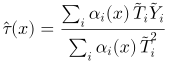
The honest-tree design reserves one half of the data to choose splits and the other half to estimate effects. That separation helps keep random noise from masquerading as a real subgroup difference. The cost is data: fine-grained variation takes a large sample to detect. If effects are constant, or the underlying relationship is linear, the forest has no advantage. Sources: [10, 11]; honest trees: [12].
AIPW (doubly robust)
AIPW pairs an outcome model  , which predicts both potential outcomes for each unit, with a weighted correction based on the outcomes actually observed. That correction gives greater influence to rare cases with low propensity.

Its appeal is real: the estimate remains correct if either the outcome model or the propensity model is correct. But extreme propensities create a sharp problem. When  approaches 0 or 1, weights
 can blow up; in Case 3, individual runs fail. AIPW estimates an average effect, and TMLE is cited as a more stable variant. Source: [13]; TMLE: [17].
2SLS with an instrument
When a confounder is unobserved, two-stage least squares can use an instrument  that shifts treatment and has no other path to outcome . The first stage extracts the treatment variation explained by the instrument. The second stage uses that predicted variation to estimate the effect, aiming to remove the influence of the hidden confounder.

With no and a binary instrument, the estimator reduces to the Wald ratio: the instrument’s effect on divided by its effect on .

Here’s the catch: the data can’t establish whether the instrument is valid. A weak instrument barely moves treatment, leaving a denominator near zero and an estimate with substantial uncertainty. Source: [5].
Instrumental forest
An instrumental forest applies the IV idea locally. For each unit , it estimates an IV effect among similar units, using forest weights . This allows the effect to vary with .
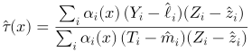
That flexibility has a price: if the effect is constant, the instrumental forest is simply noisier than 2SLS, as in Case 5. Source: [11].
Strengths and weaknesses by method
The simulation results summarize how each method performed. The guide covers which method fits which situation; this section explains why. The central choice is whether the available data and assumptions support the kind of effect you want to estimate.