Hilbert Curves Turn UK Battle Locations into a Timeline
Mapping roughly 550 UK battles across both time and geography creates a problem: each location has two coordinates, but a timeline has room for only one. A Hilbert space-filling curve offers a practical workaround, turning locations into positions along a winding path. Applied to historical battles, the result makes regional and temporal patterns easier to read. It’s a useful example of how a change in visual encoding can answer a question that a conventional map leaves crowded: when and where do events cluster together?
The source data came from Wikidata, retrieved with a SPARQL query. On a conventional map, crossed swords mark each battle. The geography hints at concentrations, including along the former borderlands of Wales, but overlapping points make the chronology harder to see. A map is good at showing where events happened; once many events occupy the same areas, it becomes less effective at showing how their locations relate to their order in time.
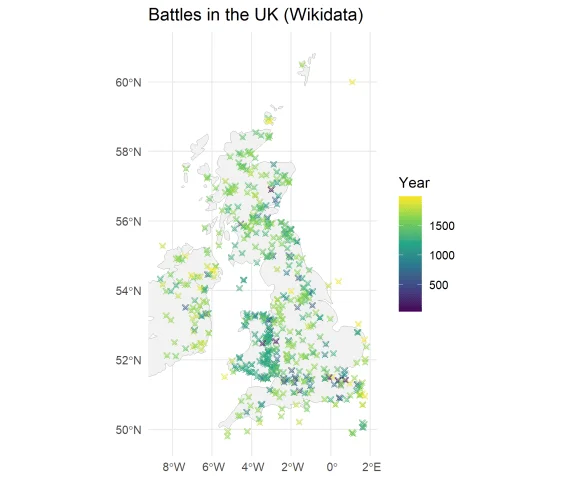
Turning a map into a line
The curve assigns each point on a two-dimensional grid a position in a one-dimensional sequence. The Hilbert curve is one way to do this: its numbered path visits every grid cell in order. Nearby positions along the curve are guaranteed to represent nearby locations on the grid, though places that are close on a map can end up far apart in the sequence. That tradeoff matters. The transformation preserves some local spatial relationships, but it can’t retain every relationship when two dimensions are compressed into one.
A Hilbert curve can be generated as a 2n by 2n matrix. In this 8-by-8 example, the numbers show the order in which the path passes through each cell:
\[\left[ \begin{matrix} 0 & 3 & 4 & 5 & 58 & 59 & 60 & 63\\ 1 & 2 & 7 & 6 & 57 & 56 & 61 & 62\\ 14 & 13 & 8 & 9 & 54 & 55 & 50 & 49\\ 15 & 12 & 11 & 10 & 53 & 52 & 51 & 48\\ 16 & 17 & 30 & 31 & 32 & 33 & 46 & 47\\ 19 & 18 & 29 & 28 & 35 & 34 & 45 & 44\\ 20 & 23 & 24 & 27 & 36 & 39 & 40 & 43\\ 21 & 22 & 25 & 26 & 37 & 38 & 41 & 42\\ \end{matrix} \right]\]Read the cells from zero upward and the sequence traces the curve. The numbering is the key to the method: each grid location gets an ordered value, which can then be plotted on an axis alongside the event’s date. The grid itself is only a way to make the mapping visible; the useful result is a shared coordinate for space and time.
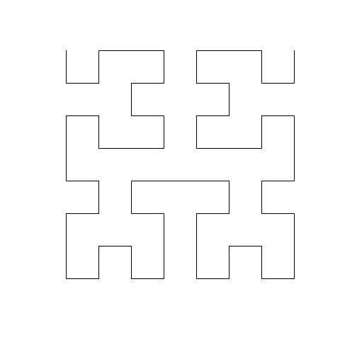
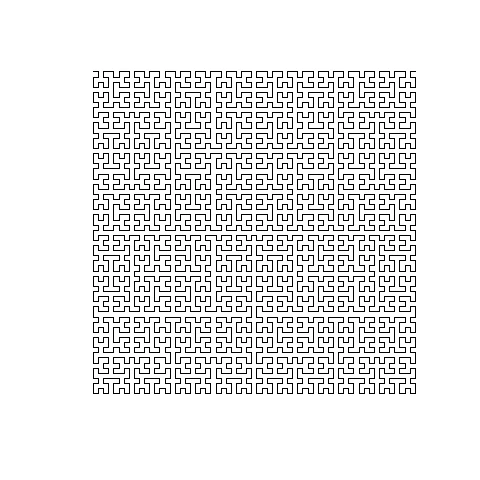
Increasing the curve’s resolution adds detail. The following illustration uses a 64-by-64 grid. A finer grid gives the encoding more distinct cells to work with, which can help when locations are close together. It also makes the mapping harder to interpret by eye, so the extra detail is valuable only if it clarifies patterns in the plotted data.
Patterns emerge in the battle record
For the UK plot, the map covers longitudes from -6 to 1.8 degrees and latitudes from 49.8 to 58 degrees. The creator added city locations for orientation and marked grid cells that were mostly sea with blue lines. Some of Ireland appears in the original data, though the chosen bounds exclude most of it. These choices shape what the visualization can show: the selected extent frames the UK record, while the sea markings help distinguish gaps in the grid from areas with no recorded battles.
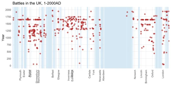
The plotted battles form three broad groups, running from left to right across the curve and corresponding approximately to Wales, Scotland and England. The encoding also gives the shape of a conflict a temporal dimension: a long run of battles around one location can appear as a vertical column, while fighting spread across a wider region can stretch horizontally. Those structures are less apparent on the original map. The result is a compact view of two kinds of concentration at once, although the curve’s ordering needs to be understood before those shapes can be read confidently.
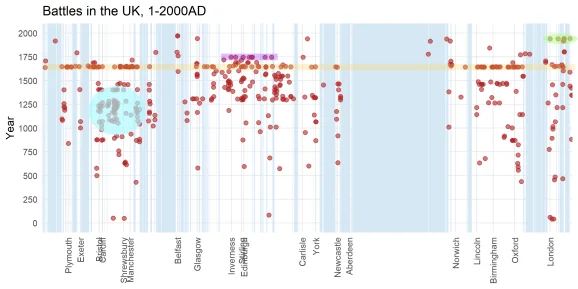
Several highlighted sequences show what the transformation can reveal. The yellow points mark battles from the English Civil War. Purple marks the Jacobite Rebellion, described in the source as the last major land battles in the UK. Turquoise traces the prolonged Conquest of Wales. Color helps separate these episodes from the full record, while their shapes show how the battles’ geographic spread relates to their sequence.
A green row near London collects several twentieth-century battles, mostly connected with the two world wars. It includes the Battle of Britain as well as naval engagements. The curve doesn’t preserve every geographic relationship, so the display works best alongside a map. Its strength is in making the combined distribution of time and place legible at a glance. If you’re working with event data, that can be a useful prompt for closer inspection, but the chart still depends on the underlying records and the choices made when plotting them.
A useful view, with an open design question
This example makes a strong case for space-filling curves as a way to inspect spatial data over time. It also leaves a practical question: when a dataset is mapped onto a curve, how should that curve be chosen to keep distortion low? The Hilbert curve gives nearby points along the sequence nearby grid locations, but it can separate places that are neighbors on the map. Finding a curve suited to a particular dataset could make this kind of view more informative. This is more significant than it looks: the curve isn’t just a technical detail, because it influences which patterns appear close and which become harder to notice.
What the visualization can and can’t tell us
The plot makes a dense record easier to scan, but a visible cluster is an invitation to investigate rather than an explanation of why battles occurred there. The encoding shows distributions and relationships; it doesn’t establish causes, and it can’t resolve the limitations of the source data. (And this is the part most people overlook.) A clean visual pattern can look more definitive than the choices behind it deserve.
That said, pairing the curve with a conventional map gives readers two complementary views: one for geographic orientation, the other for the joint sequence of time and place. The numbers here are underwhelming as a complete account of history—roughly 550 plotted battles can’t represent every conflict or every detail—but they’re enough to demonstrate the method’s value. A better-suited curve may sharpen the picture. For now, the clearest lesson is that changing the layout can expose structure without making the data itself simpler.