New R Packages Turn Complex Research Data Into Reproducible Analysis
Agriculture and causal inference
For agricultural researchers, [HRRI](https://cran.r-project.org/package=HRRI) (v1.0.9) analyzes longitudinal soil, plant, and microbial measurements during redox disturbance and recovery. It calculates potential oxygen demand and accessible electron capacity from supplied inventories and kinetic parameters, then offers recovery signatures, fixed reference domain scores, and exploratory multiblock scores with coverage diagnostics. Its methods draw on [Sander, Hofstetter and Gorski (2015)](https://doi.org/10.1021/acs.est.5b00006), [Kluepfel et al. (2014)](https://doi.org/10.1038%2Fngeo2084), and [Thompson et al. (2006)](https://doi.org/10.1016/j.gca.2005.12.005). Three vignettes are available, including [a worked guide to reading the figures](https://cran.r-project.org/web/packages/HRRI/vignettes/HRRI_gallery.html) and instructions to [reproduce all six paper figures in R](https://cran.r-project.org/web/packages/HRRI/vignettes/HRRI_paper_figures.html). [VeraCrop](https://cran.r-project.org/package=VeraCrop) (v0.1.0) automates much of the setup for comparative agricultural performance analysis: it detects variable types, preprocesses and encodes inputs, scales variables, runs diagnostics and selection, and calculates yield gaps. The approach follows [de Bie (2004)](https://doi.org/10.1016/j.scienta.2003.11.017), while [Kamkar et al. (2025)](https://doi.org/10.1016/j.agsy.2025.104392) review yield gap assessment methods. A [getting started vignette](https://cran.r-project.org/web/packages/VeraCrop/vignettes/getting-started.html) introduces the workflow.
 [phdid](https://cran.r-project.org/package=phdid) (v0.1.0) tackles a familiar tension in staggered difference in differences: estimating every cohort and time effect separately can be noisy, while pooling effects can introduce bias if they truly differ. It frames the problem as choosing a partition of cohort time cells, offering a Dirichlet process mixture fitted with a collapsed Gibbs sampler and an L0 penalized estimator that produces one partition. The methods are presented in [Arora and Wagle (2026)](https://doi.org/10.2139/ssrn.7207083). Its two vignettes examine [minimum wages and teen employment](https://cran.r-project.org/web/packages/phdid/vignettes/mpdta.html) and [when partial homogeneity helps](https://cran.r-project.org/web/packages/phdid/vignettes/simulation.html). The central practical question is whether the structure in a given study supports pooling; the package makes that choice explicit.

Climate, computation, and ecology
[xaci](https://cran.r-project.org/package=xaci) (v0.1.0) calculates the Actuarial Climate Index and its temperature, precipitation, drought, wind, and sea level components from gridded NetCDF data and tide gauge records. It adapts the French and European methodology of [Garrido, Milhaud & Olympio (2025)](https://hal.science/hal-04491982v2), building on the American Academy of Actuaries framework for use in countries worldwide. Seven vignettes include [an introduction](https://cran.r-project.org/web/packages/xaci/vignettes/xaci-intro.html) and a guide to [visualizing results](https://cran.r-project.org/web/packages/xaci/vignettes/xaci-visualization.html). Several computational releases target specialized modeling work. [koopman.dmd](https://cran.r-project.org/package=koopman.dmd) (v0.2.2) brings Dynamic Mode Decomposition and extensions of Koopman operator theory to R, with a Rust backend through
extendr. It includes standard DMD ([Schmid, 2010](https://doi.org/10.1017/S0022112010001217)), DMD with control for forced linear systems ([Proctor, Brunton, and Kutz, 2016](https://doi.org/10.1137/15M1013857)), extended DMD with lifting functions, Hankel DMD using time delay embedding, Generalized Laplace Analysis for direct eigenfunction computation, and harmonic time averages and mesochronic harmonic plots for phase space analysis, following [Mezic (2020)](https://doi.org/10.48550/arXiv.2009.05883). The [package vignette](https://cran.r-project.org/web/packages/koopman.dmd/vignettes/koopman-dmd.html) walks through its use.
[RcppTrust](https://cran.r-project.org/package=RcppTrust) (v0.1.0) offers derivative based local optimization with trust regions and a guarantee of convergence to a local minimum. It ports the algorithm from the trust package to thread safe C++, exposing both a drop in R function and a thread safe C entry point for parallel C++ code, including nlmixr2est. Its reference is the [trust package vignette](https://cran.r-project.org/web/packages/trust/vignettes/trust.pdf).
[tulpa](https://cran.r-project.org/package=tulpa) (v0.7.5) is a broader engine for Bayesian hierarchical models with spatial fields, temporal effects, and spatially varying coefficients. Spatial options include Hilbert space approximate Gaussian processes ([Riutort-Mayol et al., 2023](https://doi.org/10.1007/s11222-022-10167-2)), nearest neighbor Gaussian processes ([Datta et al., 2016](https://doi.org/10.1080/01621459.2015.1044091)), intrinsic conditional autoregressive models ([Besag, York, and Mollie, 1991](https://doi.org/10.1007/BF00116466)), the reparameterized Besag York Mollie model ([Riebler et al., 2016](https://doi.org/10.1177/0962280216660421)), and stochastic partial differential equation fields ([Lindgren, Rue, and Lindstrom, 2011](https://doi.org/10.1111/j.1467-9868.2011.00777.x)). Temporal models cover random walks, autoregressive processes, and Gaussian processes. Inference ranges from exact Hamiltonian Monte Carlo using the No U Turn sampler to Laplace and nested Laplace approximations with hyperparameter integration ([Rue, Martino, and Chopin, 2009](https://doi.org/10.1111/j.1467-9868.2008.00700.x)), plus variational inference. Model specific packages connect observation likelihoods through a templated C++ callback interface. Three vignettes include [a quick start](https://cran.r-project.org/web/packages/tulpa/vignettes/quickstart.html) and an overview of [spatial fields](https://cran.r-project.org/web/packages/tulpa/vignettes/spatial-models.html).
[WSwavelet](https://cran.r-project.org/package=WSwavelet) (v0.1.0) applies Bayesian wavelet denoising with a resolution adaptive spike and slab prior. Its continuous slab combines a compactly supported Wendland type density with the semicircle density. The package supports Gaussian and Laplace working likelihoods, empirical Bayes estimates of resolution specific slab weights, robust noise scale estimation, posterior mean coefficient shrinkage, inverse discrete wavelet reconstruction, and diagnostics. Details are in its [vignette](https://cran.r-project.org/web/packages/WSwavelet/vignettes/WSwavelet_vignette.pdf).
 Ecologists get tools for both acoustic surveys and sampling design. [acousticTS](https://cran.r-project.org/package=acousticTS) (v2.0.8) works with acoustic target strength, the intensity of echoes from individual scatterers such as bubbles, fish, or zooplankton. Target strength helps translate integrated or volumetric survey backscatter into number density, abundance, or biomass, and can help distinguish likely large predatory fish, such as adult cod, from smaller prey, such as shrimp. Applications appear in [Lucca et al. (2023)](https://doi.org/10.1121/10.0022459); background on fisheries acoustics is in [Simmonds and MacLennan (2005)](https://doi.org/10.1002/9780470995303). See the [boundary conditions vignette](https://cran.r-project.org/web/packages/acousticTS/vignettes/boundary_conditions.html).
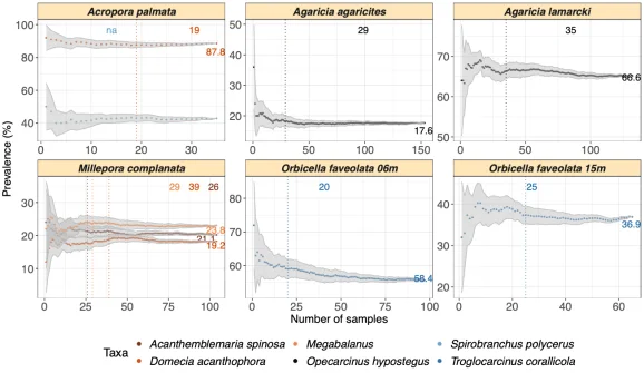
[SAMPLE](https://cran.r-project.org/package=SAMPLE) (v1.0.1) estimates how many observations are needed for stable species occurrence and prevalence estimates from presence absence data. It repeatedly subsamples observations, tracks changes in the estimated rates, and reports the minimum stable sample size. The method is described by [Bravo et al. (2025)](https://doi.org/10.1002/ece3.70998); the [GitHub repository](https://github.com/yacinebenchehida/SAMPLE) provides a starting point.
 [sptrends](https://cran.r-project.org/package=sptrends) (v1.6.3) provides reproducible inference for trends in gridded environmental time series, accounting for serial correlation, spatial dependence, and multiple testing. It includes trend preserving prewhitening, pixel level and spatially explicit inference, slope estimation, and multiple testing correction. Dedicated workflows reproduce the True Significant Trends method of [Gutiérrez-Hernández and García (2025)](https://doi.org/10.1016/j.rsase.2024.101377) and the Robust Trend Analysis method of [Gutiérrez-Hernández and García (2024)](https://doi.org/10.3390/rs16203886). Utilities cover raster import and inspection, anomaly calculation, and spatial autocorrelation diagnostics. Six vignettes include guides to [serial correlation](https://cran.r-project.org/web/packages/sptrends/vignettes/b-prewhitening.html) and [estimating trend magnitude](https://cran.r-project.org/web/packages/sptrends/vignettes/d-slope-estimation.html).

Pricing and public health
[PricingBandits](https://cran.r-project.org/package=PricingBandits) (v2.1.0) brings multi armed bandit methods to pricing experiments with an unknown demand curve, following [Weaver, Kumar, and Jain (2025)](https://doi.org/10.1287/mksc.2022.0247). It includes Upper Confidence Bound and Thompson Sampling baselines, Gaussian process models, versions that constrain demand to be weakly decreasing as price rises, and extensions for heterogeneous noise. Researchers specify willingness to pay as a vector of consumer valuations, allowing different demand environments to be simulated or replayed. The [introductory vignette](https://cran.r-project.org/web/packages/PricingBandits/vignettes/pricingbandits-intro.html) shows the workflow. In epidemiology, [ambre](https://cran.r-project.org/package=ambre) (v2.1.2) models quantitative microbial risks when treated wastewater is reused for agricultural irrigation. Its multi barrier approach simulates pathogen inflow and removal through a treatment train, estimates human exposure, and calculates infection and illness probabilities plus Disability Adjusted Life Years. It can also compare treatment scenarios economically. The work is detailed by [Thomas et al. (2024)](https://doi.org/10.36904/20240595), and eight vignettes include [a getting started guide](https://cran.r-project.org/web/packages/ambre/vignettes/a-get-started.html) and guidance on [interpreting risk against the WHO target](https://cran.r-project.org/web/packages/ambre/vignettes/d-interpreting-risk.html).
 [tbl.now](https://cran.r-project.org/package=tbl.now) (v1.2.0) defines tidy data structures and package independent workflows for epidemiological nowcasting. Its
tbl_now class stores event, report, and revision dates, along with strata, covariates tagged by model component, censoring, and reporting delay metadata, while remaining compatible with dplyr. Tools cover validation, data manipulation, diagnostics, visualization, conversion, retrospective evaluation, and connections to multiple modeling engines. See the [vignette](https://cran.r-project.org/web/packages/tbl.now/vignettes/tbl.now.html).

Genomics and machine learning
mSigSpectra v0.1.3 tackles a practical genomics problem: turning variant calls into comparable mutation catalogs without tying the workflow to one variant caller. It reads VCF files, adds flanking-sequence and transcriptional-strand annotations, then summarizes single-base substitutions, doublet substitutions, and small insertions and deletions. Researchers can choose among ten catalog resolutions—SBS96, SBS192, SBS1536, DBS78, DBS136, DBS144, ID83, ID89, ID166, and ID476—and represent results as either counts or densities. The package was used to prepare Rozen et al. (2026); its vignette explains the workflow.

Machine learning
The appeal of fastgbm v0.6.1 is breadth under one interface. It handles regression with squared error, binary and multiclass classification with logistic and one-vs-rest approaches, and right-censored survival data. For survival analysis, users can choose Cox objectives with Breslow ties, normal location-scale accelerated failure time, or piecewise-exponential objectives. The package also routes missing values natively, estimates baseline hazards, predicts survival probabilities, and trains deterministically across threads with RcppParallel. The methods build on Friedman (2001). Six vignettes are available, including Getting Started and an algorithm guide.

Interpretability is the focus of xplaineff v0.1.1, which implements the Generalized Additive Decomposition of Global EffecTs algorithm. It recursively divides feature space into regions where effects are less heterogeneous, building a tree that can expose where a feature’s influence changes. Users can choose Accumulated Local Effects or Partial Dependence strategies, connect the method to mlr3 learners, and inspect both the interaction tree and regional effect plots. That offers a useful way to qualify global effect summaries, though the resulting regions still need interpretation in the context of the model and data. The approach is described by Herbinger et al. (2024); see the vignette.

Medical statistics and meta-analysis
chms v7.2 packages the ActiGraph wGT3X-BT accelerometer processing workflow used by Statistics Canada for cycle 7 of the Canadian Health Measures Survey. Its value is methodological consistency: researchers can follow a documented, reproducible process and align analyses with the agency’s approach. The general methods are described in Clarke et al. (2026), with setup guidance in the README.
For sequential multiple assignment randomized trials, rsmart v0.1.0 implements an interim augmented inverse probability weighted estimator of treatment-regime value. The estimator encompasses both inverse probability weighting and augmented inverse probability weighting, supporting inference at interim and final analyses. Its tools cover value estimation, sandwich variance, group-sequential stopping boundaries, and sample-size calculations for multi-stage SMARTs. The underlying work is detailed by Manschot, Laber, and Davidian (2023). Four vignettes include Getting Started and a full IAIPWE demonstration.

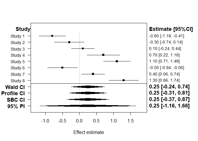
metaGLMM v1.0.0 brings random-effects meta-analysis into a generalized linear mixed-effects model framework. That lets analysts work with aggregate data while adjusting for covariates and handling non-normal responses; likelihood-based inference is paired with computationally efficient likelihood evaluation. The methodology comes from Hanada and Sugimoto (2026). Seven vignettes cover the package, including Getting Started and prediction and forest plots.
Networks and phylogenetics
nethist v1.0.0 estimates network histograms, blockmodel approximations to the graphon that describes a network’s connectivity. It supports single-layer and multilayer networks, drawing on the profile-likelihood method of Olhede and Wolfe (2014) and the least-squares method of Gao, Lu, and Zhou (2015) for single-layer cases, alongside the multilayer extension by Song and Olhede (2026). The vignette provides an example.

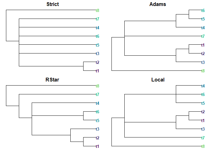
Consensus trees come in several flavors, and ConsTree v1.0.0 makes a broad set of them available for efficient construction. Supported methods include strict, majority-rule, majority-rule (+), loose (combinable component, semi-strict), greedy, Adams, frequency difference, R*, and local consensus. A vignette walks through the package.
Statistical methods
Missing outcomes can make randomized experiments hard to interpret when the missingness process is nonignorable. attrition v1.0.0 implements the double-sampling bounds estimator from Coppock et al. (2017). It also calculates worst-case Manski bounds and double-sampling bounds with analytic variance and Imbens-Manski confidence intervals. For Lee (2009) trimming bounds, it offers analytic and bootstrap standard errors; further options include poststratification adjustment and sensitivity analysis for departures from the outcome-stability assumption. The original method is described by Lee (2009), and the package’s vignette shows how to use it.

Distribution fitting can become a selection problem of its own. FitVerse v1.0-2 offers a common interface for continuous univariate data across 52 families, from symmetric and bounded distributions to right-skewed, heavy-tailed, and extreme-value forms. It supports three estimation methods and ranks candidate fits using multiple criteria and tests. The package adds diagnostic plots, histograms with density overlays, optional interactive plotly views, bootstrap confidence intervals for parameters and return levels, and batch fitting across columns. Those features suit survey sampling, hydrology, and actuarial work. For background, see Hosking (1990) and the FitVerse vignette.

For panel data with interactive fixed effects, hdcce v0.1.0 implements estimation and inference for both the linear specification in Ruecker, Vogt, Linton, and Walsh (2025) and the dictionary design in Ruecker, Vogt, and Linton (2026). Details are in the vignette.
HDElliptical v0.1.3 collects methods for robust estimation, testing, dimension reduction, classification, and clustering when data are high-dimensional and elliptically symmetric. Its computational kernels use Rcpp and RcppArmadillo. The methods are reviewed in Feng (2026); two starting points are the vignettes on robust directional foundations and location tests.
Ordered outcomes sometimes contain a category populated by two distinct processes. iop v0.1.0 estimates ordered probit and logit models for this case, where an inflated category mixes observations from the ordinary ordered process with those from a separate split-population process. It implements the zero-inflated ordered probit of Harris and Zhao (2007), plus middle- and top-inflated extensions such as those discussed by Bagozzi, Joo and Mukherjee (2024). Available features include analytic, robust, and cluster-robust standard errors, survey weights, offsets, model comparisons, regime-specific predicted probabilities, and first differences. Four vignettes include Getting Started and a guide to the model, identification, and estimation.
normalblockr v0.3.0 changes the unit of network analysis: its Normal-Block model clusters variables, then estimates dependencies between clusters rather than between every pair of individual variables. The Gaussian graphical model builds on the graphical lasso and supports known or unknown cluster assignments, with an optional zero-inflation extension for data containing many exact zeros. The model and its variational expectation-maximization procedure are described by Tous & Chiquet (2026). Four vignettes include examples of Mean-Block models and zero-inflated Normal-Block models.
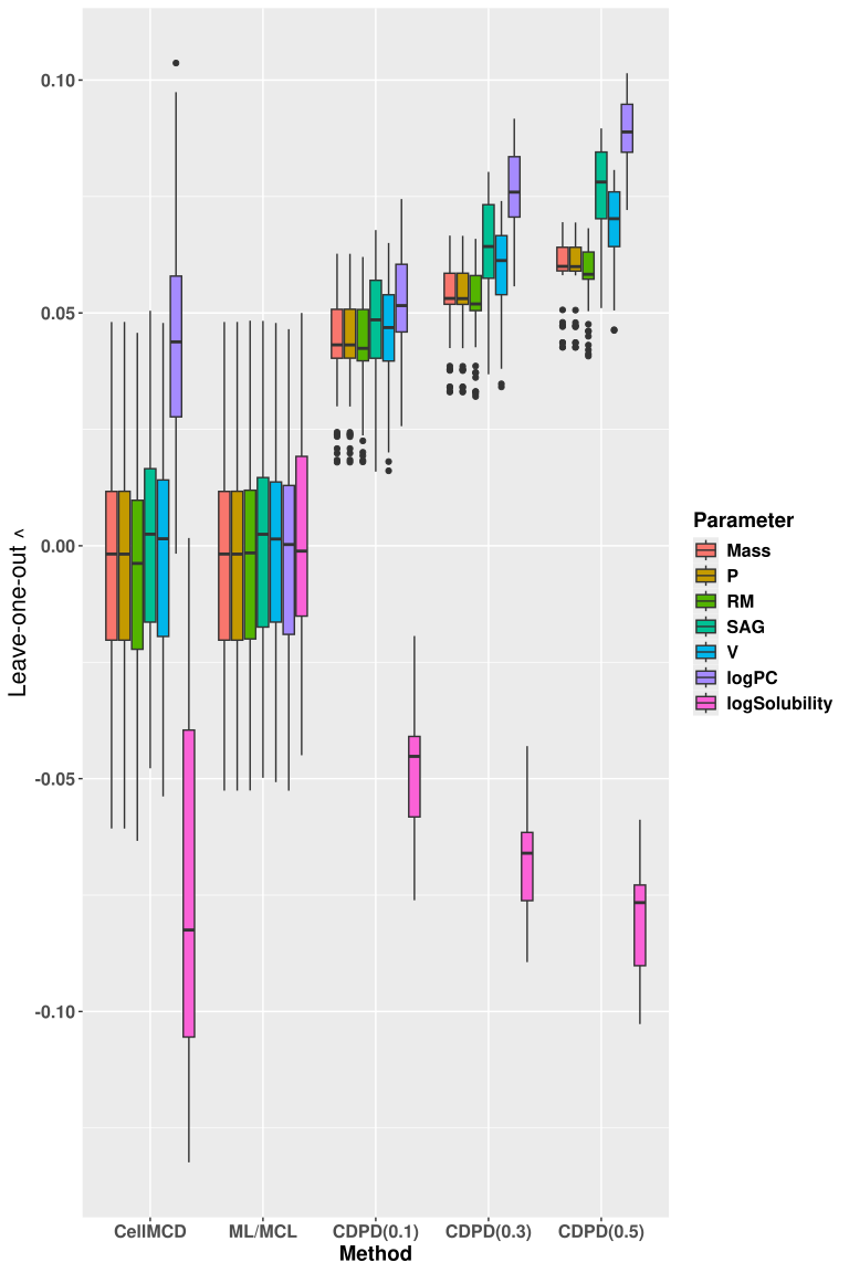
mvdpd v0.1-1 applies multivariate Density Power Divergence methods to robust estimation. It covers multivariate normal models under casewise and cellwise contamination, using multivariate, composite, or componentwise minimization, and also offers robust estimation for multivariate ordered gamma models with multivariate and composite DPD minimization. The details are in Ghosh, Agostinelli, and Basu (2026). Examples are available for mvnormDPD and mvogammaDPD.
How much data does a prediction model need? pmsims v1.0.0 approaches that question through repeated simulation: generate data, fit models, and measure how sample size affects predictive accuracy, calibration, and overfitting. It supports continuous, binary, and time-to-event outcomes, as well as regression and machine-learning methods. The methods appear in Olaniran et al. (2026) and Shamsutdinova et al. (2026); the vignette shows the workflow.

Models for high-dimensional data
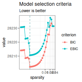
spfcICOMP v0.1.0 tackles dimension reduction for high-dimensional regression and classification through shrinkage principal fitted components. It combines regularized covariance estimates—using Oracle Approximating Shrinkage and Maximum Entropy Covariance—with response-guided feature screening, structural-dimension selection, reduced-space prediction and simulation tools. Users can choose conventional or information-complexity criteria for selecting the structural dimension. The methods draw on Cook and Forzani (2008), Chen et al. (2010), Bozdogan (2000) and Olorede and Yahya (2019). The getting-started vignette is the place to see how those pieces fit together.
For count data with spatial or temporal structure, ZINB.GP v1.0.0 fits Bayesian zero-inflated negative binomial models with Gaussian process random effects. It supports spatial, temporal and spatiotemporal data, Markov chain Monte Carlo sampling, configurable random effects in both the zero-inflation and count components, and posterior predictive draws. The package implements a full Gaussian process version of methods from He and Huang (2024). The examples cover Oregon landslides and simulating and fitting a spatiotemporal ZINB-GP model.

Surveys
Survey response rates alone don’t tell you whether the people who answered represent the population you meant to reach. risq v3.0.1 calculates representativity indicators from survey data and response models, including R-indicators and coefficients of variation. Its partial indicators help isolate the effects of particular variables or categories; during collection, those measures can track changing representativity and inform adaptive survey design. The package’s foundations include Schouten, Cobben and Bethlehem (2009), Shlomo, Skinner and Schouten (2012) and Schouten and Shlomo (2017). Its introduction and theory vignette explain the measures and their use.
Utilities
Data lineage is easier to inspect when it’s visible. dplyneage v0.3.1 turns dplyr and dbplyr pipeline transformations into column-lineage visualizations with React Flow, using an interface familiar to tidyverse users. Its guides cover getting started with dplyneage and building the React Flow bundle.

For R users working with lakehouse data, ducklake v0.6.0 brings a tidyverse-friendly interface to DuckLake, the DuckDB lakehouse format. You can attach versioned data lakes and use familiar dplyr verbs while retaining ACID transactions, time-travel queries, snapshot audit trails, data inlining and encrypted storage. Catalog options include DuckDB, PostgreSQL, SQLite and MySQL; remote access is also supported over DuckDB’s ‘Quack’ protocol. There are nine vignettes, including the ducklake Cookbook and Time Travel Queries.
External data dependencies can undermine reproducibility when they change or disappear. getaca v0.1.6 provides functions to declare, retrieve, verify, track and actively manage resources that are too large or fast-moving to bundle with an R package. Each resource is identified by package, name and version, pinned with a SHA-256 checksum, and resolved under an explicit policy so an installed package gets the same bytes each time. A remote registry can also carry an Ed25519 signature checked against a key shipped by the declaring package, keeping the registry and its validating key on separate routes. The design targets reproducible offline use and graceful behavior during package checks. Among its eight vignettes are Quick Start and Policies and Channels.
icebergr v0.2.0 offers R a native client for Apache Iceberg, an open table format used by Snowflake, Databricks, BigQuery, AWS and Dremio. It connects to REST and AWS Glue catalogs; lists namespaces and tables; reads table schemas and partition specifications; and scans data with predicate and projection pushdown. It can also traverse snapshot history and append data, with Apache Arrow serving as the interchange layer. Iceberg support can vary considerably by feature, so consult the package’s README and support matrix for what works and what doesn’t. Seven vignettes include Getting Started and What Iceberg Is, and What It Fixes.

Package review quality depends on checks that reach beyond whether code runs. pkgcheck v0.3.4 assesses whether a package is ready for submission to the rOpenSci peer-review system. It builds on goodpractice and adds checks, including ones focused on maintaining public online code repositories. The current checks and guide to adding or modifying checks show how the system can be applied and extended.
Visualization
Statistical graphics have a history worth borrowing from. ggCheysson v1.1.0 brings the fonts, hatched patterns and color palettes associated with Emile Cheysson’s Albums de Statistique Graphique to ggplot2. The albums are sometimes described as the pinnacle of the Golden Age of Statistical Graphics; the package makes those stylistic choices available for contemporary plots. Its three vignettes include Getting Started and Mapping Guerry’s Moral Statistics with Cheysson Palettes.

Taken together, these releases show R packages reaching across the full workflow: statistical modeling, survey quality, data provenance, lakehouse access, package review and visual presentation. The more consequential shift may be the attention to reproducibility and traceability—concerns that matter just as much as adding another modeling method when analyses depend on external data and complex pipelines.