You Don’t Need to Learn All the Weights on tabular data: The Case for rvflnet (a nonlinear expressive glmnet) on regression, classification and survival analysis

Introduction

Random Vector Functional Link (RVFL) networks offer a simple yet powerful alternative to traditional neural networks for tabular data. Instead of learning hidden layers through backpropagation, RVFL generates them randomly (or not, if using a deterministic sequence of quasi-random numbers) and focuses all learning effort on a final, regularized linear model.

Formally, let

\[X \in \mathbb{R}^{n \times p}\]

be the input data. RVFL networks (the ones described in this blog post) construct a set of nonlinear features by projecting (X) onto a random matrix

\[W \in \mathbb{R}^{p \times m},\]

and applying an activation function (\(g(\cdot)\)):

\[H = g\left( \frac{X – \mu}{\sigma} ; W \right).\]

These random nonlinear features are then concatenated with the original inputs to form an augmented design matrix:

\[Z = [X | H].\]

The model prediction is obtained by fitting a linear model on this expanded space (hence, a nonlinear GLM):

\[\hat{y} = Z \beta.\]

Because (Z) can be high-dimensional and highly redundant, RVFL networks (the ones described in this blog post) rely on Elastic Net regularization (glmnet) to estimate the coefficients:

\[\hat{\beta} = \arg\min_{\beta}\mathcal{L}(y, Z\beta) + \lambda \left(\alpha ||\beta||_1 + (1-\alpha)||\beta||_2^2\right).\]

In this framework, randomness creates a rich pool of nonlinear transformations, while regularization selects and stabilizes the most useful ones. The result is a nonlinear model that combines the flexibility of neural networks with the efficiency and robustness of linear methods.

Of course, this blog post is not a proof of the title. It’s about R package rvflnet. But you can appreciate the high performance of RVFLs on regression, classification and survival analysis, an notably on the controversial Boston dataset (performs on par with Random Forest or Gradient Boosting).

0 – Install package

install.packages("survival", repos = "https://cran.r-project.org") # survival analysis
install.packages("remotes", repos = "https://cran.r-project.org")
devtools::install_github('thierrymoudiki/rvflnet') # Nonlinear glm (RVFL networks)

1 – Regression

set.seed(123)
library(glmnet)
data(Boston, package = "MASS")
# -------------------------
# Data
# -------------------------
X <- as.matrix(Boston[, -14])
y <- Boston$medv
n <- nrow(X)
idx <- sample(1:n, size = round(0.8 * n))
X_train <- X[idx, ]
y_train <- y[idx]
X_test <- X[-idx, ]
y_test <- y[-idx]
# -------------------------
# Grid
# -------------------------
grid <- expand.grid(
n_hidden = c(175, 200, 225, 250),
alpha = seq(0.1, 0.5, by=0.2),
include_original = c(TRUE, FALSE),
seed = 1,
stringsAsFactors = FALSE
)
results <- vector("list", nrow(grid))
# -------------------------
# Loop
# -------------------------
for (i in seq_len(nrow(grid))) {
params <- grid[i, ]
#cat("\n========================================\n")
#cat(sprintf("Run %d / %d\n", i, nrow(grid)))
#print(params)
# -------------------------
# Fit model
# -------------------------
fit <- rvflnet::rvflnet(
X_train, y_train,
n_hidden = params$n_hidden,
activation = "sigmoid",
W_type = "gaussian",
seed = params$seed,
include_original = params$include_original, # direct link, skip connection or not
alpha = params$alpha
)
# -------------------------
# Evaluate full lambda path
# -------------------------
lambdas <- fit$fit$lambda
preds <- predict(fit, newx = X_test, s = lambdas)
rmse_path <- sqrt(colMeans((preds - y_test)^2))
best_idx <- which.min(rmse_path)
best_rmse <- rmse_path[best_idx]
best_lambda <- lambdas[best_idx]
# -------------------------
# Sparsity
# -------------------------
coef_mat <- coef(fit, s = best_lambda)
nonzero <- sum(coef_mat[-1, 1] != 0)
# -------------------------
# Verbose output
# -------------------------
#cat(sprintf("Best RMSE: %.4f\n", best_rmse))
#cat(sprintf("Best lambda: %.6f\n", best_lambda))
#cat(sprintf("Non-zero coeffs: %d\n", nonzero))
# -------------------------
# Store
# -------------------------
results[[i]] <- data.frame(
n_hidden = params$n_hidden,
alpha = params$alpha,
include_original = params$include_original,
seed = params$seed,
rmse = best_rmse,
lambda = best_lambda,
nonzero = nonzero
)
}
# -------------------------
# Aggregate
# -------------------------
results_df <- do.call(rbind, results)
results_df <- results_df[order(results_df$rmse), ]
print(head(results_df))
Loading required package: Matrix
Loaded glmnet 4.1-10
n_hidden alpha include_original seed rmse lambda nonzero
s= 0.027561759 200 0.1 TRUE 1 2.881935 0.02756176 190
s= 0.017620327 200 0.3 TRUE 1 2.884739 0.01762033 167
s= 0.012734248 200 0.5 TRUE 1 2.889339 0.01273425 158
s= 0.036435024 175 0.1 TRUE 1 2.920012 0.03643502 165
s= 0.016833926 175 0.5 TRUE 1 2.938472 0.01683393 136
s= 0.023293035 175 0.3 TRUE 1 2.941267 0.02329304 144

An RMSE of 2.88 is on par with Random Forest or Gradient Boosting, with a significantly faster computation time.

2 - Classification

2 - 1 Binary Classification

set.seed(123)
data(iris)
# Binary classification: setosa vs others
y <- ifelse(iris$Species == "setosa", 1, 0)
X <- as.matrix(iris[, 1:4])
# Train/test split
n <- nrow(X)
idx <- sample(1:n, size = round(0.8 * n))
X_train <- X[idx, ]
y_train <- y[idx]
X_test <- X[-idx, ]
y_test <- y[-idx]
# -------------------------
# Fit model
# -------------------------
cv_model <- rvflnet::cv.rvflnet(
X_train, y_train,
n_hidden = 50,
activation = "relu",
W_type = "gaussian",
family = "binomial",
nfolds = 5
)
# -------------------------
# Predictions (probabilities)
# -------------------------
(probs <- predict(cv_model, X_test, type = "response"))
# Convert to class
y_pred <- ifelse(probs > 0.5, 1, 0)
all.equal(as.numeric(y_pred), as.numeric(predict(cv_model, X_test, type="class")))
# -------------------------
# Diagnostics
# -------------------------
# Accuracy
acc <- mean(drop(y_pred) == y_test)
cat("Accuracy:", acc, "\n")
# Confusion matrix
table(Predicted = y_pred, Actual = y_test)

A matrix: 30 × 1 of type dbl

lambda.min
0.9997617002
0.9992267955
0.9997120678
0.9997524867
0.9996600481
0.9992472082
0.9996101744
0.9999356520
0.9998139568
0.9995418762
0.0003328885
0.0003328885
0.0003328885
0.0019937012
0.0003328885
0.0005459970
0.0003328885
0.0005035848
0.0003328885
0.0003328885
0.0003328885
0.0003328885
0.0003328885
0.0003328885
0.0003328885
0.0003328885
0.0003328885
0.0003328885
0.0003328885
0.0003328885

TRUE

Accuracy: 1
Actual
Predicted 0 1
0 20 0
1 0 10

2 - 2 Multiclass Classification

set.seed(123)
data(iris)
y <- as.numeric(iris$Species)
X <- as.matrix(iris[, 1:4])
# Train/test split
n <- nrow(X)
idx <- sample(1:n, size = round(0.8 * n))
X_train <- X[idx, ]
y_train <- y[idx]
X_test <- X[-idx, ]
y_test <- y[-idx]
# -------------------------
# Fit model
# -------------------------
cv_model <- rvflnet::rvflnet(
X_train, y_train,
n_hidden = 50,
activation = "relu",
W_type = "gaussian",
family = "multinomial",
nlambda = 25,
nfolds = 5
)
# -------------------------
# Diagnostics
# -------------------------
# Accuracy
acc <- colMeans(predict(cv_model, X_test, type="class") == y_test)
cat("Accuracies:", acc, "\n") # consider other metrics
Accuracies: 0.1666667 0.7666667 0.9333333 0.9666667 0.9666667 0.9666667 0.9666667 0.9666667 0.9666667 0.9666667 0.9666667 0.9666667 0.9666667 0.9666667 0.9666667 0.9666667 0.9666667 0.9666667 0.9666667 0.9666667 0.9666667 0.9666667 0.9666667

3 - Nonlinear Cox survival analysis

3 - 1 Example 1

library(survival)
library(rvflnet)
data(ovarian)
X <- as.matrix(ovarian[, c("age", "resid.ds", "rx", "ecog.ps")])
y <- Surv(ovarian$futime, ovarian$fustat)
set.seed(123)
n <- nrow(X)
train_idx <- sample(1:n, size = round(0.8 * n))
X_train <- X[train_idx, ]
X_test <- X[-train_idx, ]
y_train <- y[train_idx]
y_test <- y[-train_idx]
# -------------------------
# Fit model
# -------------------------
cv_fit <- rvflnet::cv.rvflnet(
X_train, y_train,
family = "cox",
nfolds = 5,
type.measure = "C"
)
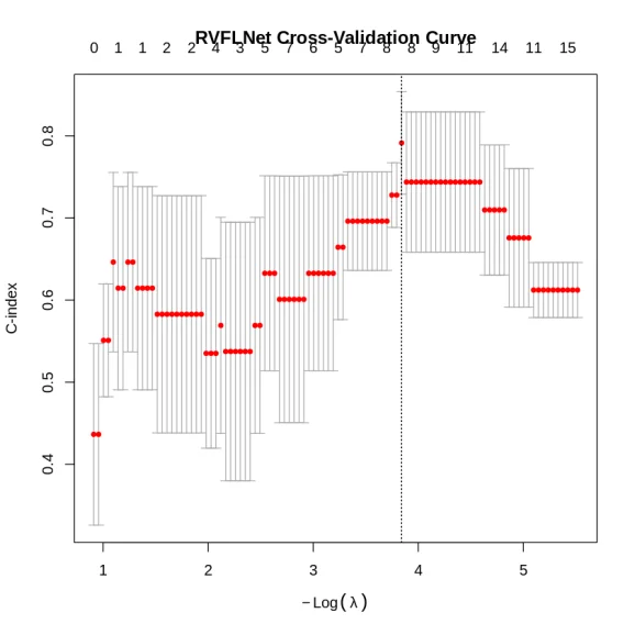
plot(cv_fit)
# Out-of-sample C-index
print(glmnet::Cindex(pred = predict(cv_fit, X_test), y = y_test))
Warning message in data(ovarian):
“data set ‘ovarian’ not found”
[1] 0.8571429

3 - 2 Example 2

library(glmnet)
library(survival)
data(pbc)
pbc2 <- pbc[!is.na(pbc$trt), ]
pbc2$event <- as.integer(pbc$status[!is.na(pbc$trt)] == 2)
pbc2$sex_n <- as.integer(pbc2$sex == "f")
feat_cols <- c("trt","age","sex_n","ascites","hepato","spiders","edema",
"bili","chol","albumin","copper","alk.phos","ast",
"trig","platelet","protime","stage")
df <- pbc2[, c("time", "event", feat_cols)]
for (col in feat_cols)
if (any(is.na(df[[col]])))
df[[col]][is.na(df[[col]])] <- median(df[[col]], na.rm = TRUE)
set.seed(42)
idx_train <- sample(nrow(df), floor(0.75 * nrow(df)))
train <- df[idx_train, ]; test <- df[-idx_train, ]
X_tr <- as.matrix(train[, feat_cols])
X_te <- as.matrix(test[, feat_cols])
y_tr <- Surv(train$time, train$event)
fit <- rvflnet::rvflnet(
X_tr, y_tr,
family = "cox",
alpha=0.1, lambda=0.1 # not recommended
)
y_te <- Surv(test$time, test$event)
ci <- glmnet::Cindex(predict(fit, X_te), y_te)
cat("\n=== Test-set C-index ===\n")
print(ci)
=== Test-set C-index ===
[1] 0.8218117
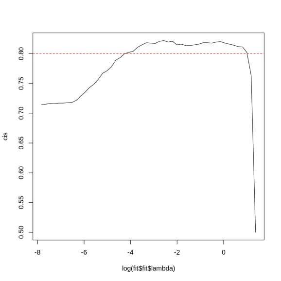
fit <- rvflnet::rvflnet(
X_tr, y_tr,
family = "cox",
alpha=0.1, nlambda=50
)
y_te <- Surv(test$time, test$event)
(cis <- apply(predict(fit, X_te), 2, function(x) glmnet::Cindex(x, y_te)))
#cat("\n=== Test-set C-index ===\n")
plot(log(fit$fit$lambda), cis, type = 'l')
abline(h=0.8, lty=2, col="red")

s0

0.5

s1

0.762812872467223

s2

0.802145411203814

s3

0.811084624553039

s4

0.811680572109654

s5

0.814064362336114

s6

0.815852205005959

s7

0.817640047675805

s8

0.820023837902265

s9

0.81942789034565

s10

0.817640047675805

s11

0.81823599523242

s12

0.81823599523242

s13

0.815852205005959

s14

0.814660309892729

s15

0.813468414779499

s16

0.813468414779499

s17

0.815852205005959

s18

0.814660309892729

s19

0.82061978545888

s20

0.81942789034565

s21

0.82181168057211

s22

0.82061978545888

s23

0.817044100119189

s24

0.817640047675805

s25

0.81823599523242

s26

0.814660309892729

s27

0.810488676996424

s28

0.803933253873659

s29

0.802145411203814

s30

0.799761620977354

s31

0.793206197854589

s32

0.789034564958284

s33

0.777711561382598

s34

0.771156138259833

s35

0.766984505363528

s36

0.756853396901073

s37

0.748510131108462

s38

0.743146603098927

s39

0.735399284862932

s40

0.728843861740167

s41

0.721692491060787

s42

0.718116805721096

s43

0.717520858164482

s44

0.716924910607867

s45

0.716924910607867

s46

0.715733015494636

s47

0.716328963051251

s48

0.715137067938021

s49

0.713945172824791

Continue reading: You Don’t Need to Learn All the Weights on tabular data: The Case for rvflnet (a nonlinear expressive glmnet) on regression, classification and survival analysis